Plotting
This section summarises the various plotting options that are offered.
Table of contents
Main UI elements
Once an H5parm has been loaded the UI opens. A number of options are available here. At the top serveral drop-down menus handle data selection. Below that several checkboxes control how the data is plotted. A scrollable list showing all the antennas present in the solutions sets which antenna to plot. The drop-down menus are explained in the table below.
| Menu | Purpose |
|---|---|
| SolSet | Selects the solution set to retrieve SolTabs from. Defaults tot he first SolSet found. |
| Plot | Selects the SolTab to plot. Defaults to the first SolTab found. |
| vs | Determines whether to plot the quantity against time, frequency or as a waterfall plot, if supported. Defaults to time. |
| Ref. Ant. | Sets the reference antenna for phase(-like) quantities. Instead of plotting the raw values, it plots data - data_ref. This has no effect on amplitude data. |
| Dir. | Selects the direction to plot if multiple directions are present in the selected SolTab. |
The plot button will open a new window plotting the solutions of the selected station. The Next antenna and Previous antenna iterate over antennas within a plot window. For 1D plots, if multiple time or frequency slots are available then the scrollbar or Forward and Backward buttons allow one to scrub the time or frequency axis. For 2D waterfall plots these buttons iterate over polarisations when applicable. Each plot window is independent of the others, meaning modifiers and iterations are specific to itself and will not affect other plots.
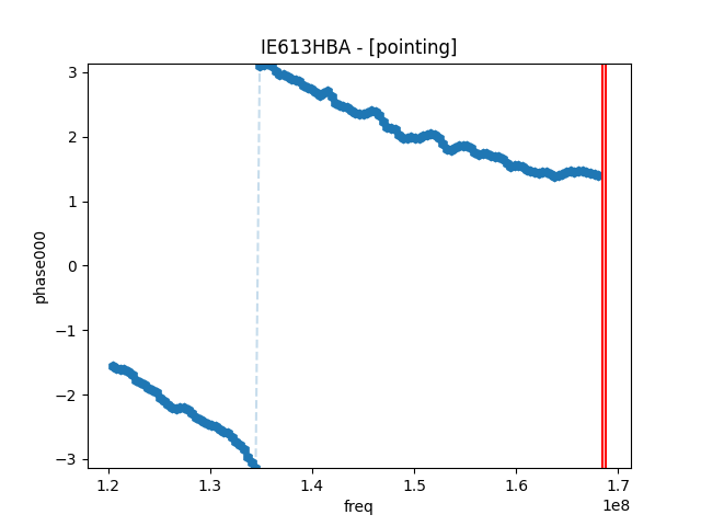
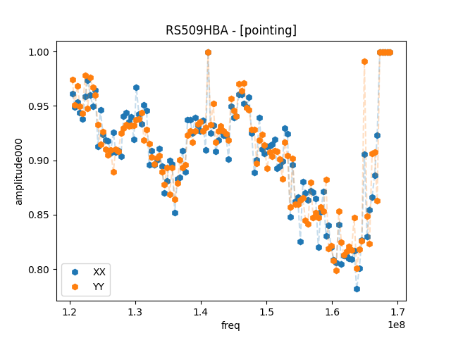
1D plots
1D plots are your every day x-y plots. It plots the selected quantity versus time or frequency. If multiple polarisations are present they are plotted simultaneously. When solutions are plotted as function of time it is possible to iterate over frequency by means of the “forward” and “backward” buttons, or the scrollbar.
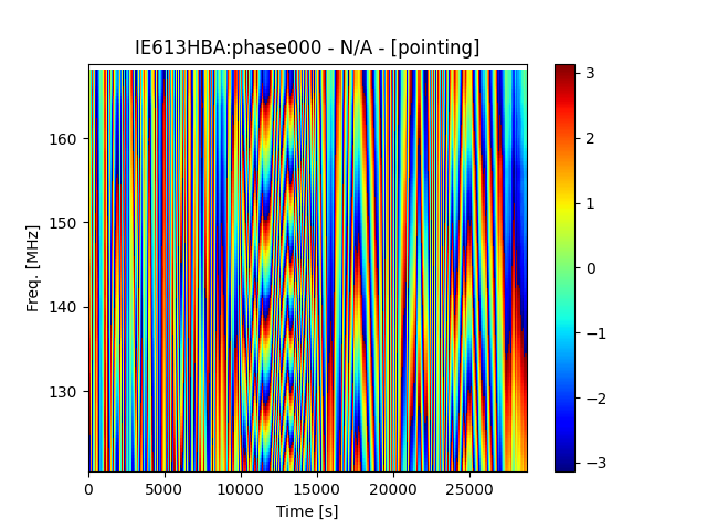
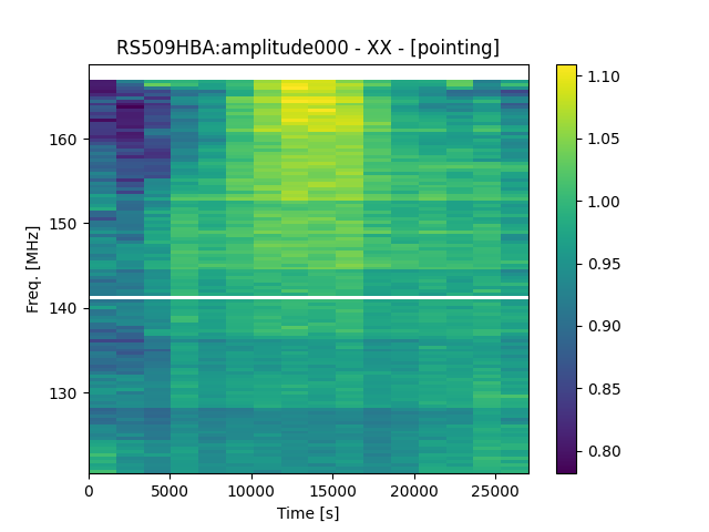
2D plots
2D plots, also called “dynamical spectrum” or “waterfall” plots can be made by selecting the “waterfall” option instead of time or frequency. In this case a two-dimensional plot will be generated showing frequency against time where the colour scale indicates the value of the quantity of interest. If multiple polarisations are present, they can be iterated over using the “forward” and “backward” buttons.
Advanced plotting options
A number of options modify the plotting behaviour. These can be useful for more specialised inspections.
Weights
H5parms have weights associated to their values that indicate whether they are flagged (weight == 0) or not (weight == 1). Ticking the “Plot weights” checkbox will plot these weights instead of the values. This can give a quick indication of which solutions have been flagged.
Discrete difference
The “Time diff.” and/or “Freq. diff.” checkboxes will change plotting behaviour such that the first discrete difference is plotted instead of the data itself, plotting data[i+1] - data[i] along the respective axes.
Polarisation difference
The “Pol. diff.” checkbox plots the difference between the XX and YY polarisations.